Fourier Transform for Digital Image Processing

Go to Index

I studied computer science (BSc.) at a technical university. The Fourier transform subject appeared at least three times on various courses (basics of electronics, calculus 2, networking technologies). I don't know, maybe it's just me, but I think the lecturers didn't pay enough attention to this subject and they didn't explain it. You know, they were either excited with formulas (which at that time had no sense to me) without letting us understand what is actually going on, or they though that we had already understood that subject before so they were doing short remainders, also without much explanation. The result was that I finished my studies and I didn't know what is Fourier transform actually for and, hold me, how to actually compute it numerically.

Obviously, it's not only the fault of the lecturers that I didn't understand Fourier transform. It was also my fault because I didn't consider it important - I thought it was a concept that only people dealing with electronics are concerned. I was wrong. I eventually found out that Fourier transform plays a vital role in digital image processing. However, to better understand using Fourier transform on images, it's better to have some intuition with traditional 1-D functions.

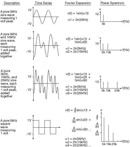
Ok, let's finally say what intuitively Fourier transforms does. Once upon a time, a fellow called Jean Fourier discovered, that a vast majority of functions can be approximated with a finite sum of sines and cosines (in inifnity, a function can be exactly expressed with sines and cosines) (http://www.files.chem.vt.edu/chem-ed/data/graphics/fourier-waves.gif). Take a look here: http://brokensymmetry.typepad.com/photos/uncategorized/2008/06/19/transform_pairs_3.gif. Note the 3rd illustration, which depicts a sine function on the left in time domain. On the right we can see its Fourier transform (only its Real value - more on this in the next paragraph), that is, the sine function transformed to frequency space. Note that the function consists of exactly one frequency, namely $2\pi$ (present at point $f = \frac{1}{T} = \frac{1}{2\pi}$). This also explains why various forms of Fourier transform are used in data compression. Here, knowing a single value (the frequency) we can easily reconstruct the original function in time domain! Of course, various functions have various representations in frequency domain. Note for example how the boxcar's Fourier transform looks like.

One basic thing we must remember is that Fourier transform operates not on real, but on complex numbers! That is, it takes as input a set of complex numbers and outputs a set of complex numbers. Naturally, since we deal with real functions in time domain, their complex values have imaginary parts equal to $0$. However, on the output, the Fourier transform will in general yield complex values. And this is good! This way we can know what the amplitudes are:
\begin{eqnarray}
amplitude = \sqrt{real*real + imaginary*imaginary}
\end{eqnarray}
and what the phases are:
\begin{eqnarray}
phase = \mbox{atan2}(imaginary, real)
\end{eqnarray}
And now yet another important thing. In this link http://www.dataq.com/images/article_images/fourier-transform/an11fig1.gif on the right there are plots of power spectrum values (these are usually Ampltiude*Amplitude, but the sole Amplitude is also often plotted). We usually skip phases and plot amplitudes because we are usually more interested in how "big" particular frequencies are, and not how much they are offset.

One intuition we need to have is how, more or less, the Fourier transform of a particular function can look like. Roughly speaking, if a function is smooth and don't have any sudden height variations, it will have only low/medium frequencies, but not high. On the other hand, if a function has sharp and sudden variations in values, its Fourier transform will depict high frequencues. Note that, for example, noises are high-frequency phenomenons. This is one of the most fundamental applications of Fourier transform - removal of noises. We can take the Fourier transform of a signal/function, eliminate high frequencies (noises mostly) and use inverse Fourier transform to get the input signal without noises.

Okay, so how does it all translate to image processing? Roughly speaking, here we have a 2-dimensional function given in spatial domain (it's a counterpart of 1D time domain) where pixels' intensities form the input function (think of a whole bunch of functions, each one representing a single row of pixels). This can be used as input to the Fourier transform. Now I stop talking and point valuable Internet resources where you can grab a vast of useful information, including source codes showing implementation of Fourier transform:
http://www.cs.otago.ac.nz/cosc453/student_tutorials/fourier_analysis.pdf
http://homepages.inf.ed.ac.uk/rbf/HIPR2/fourier.htm
http://www.cs.unm.edu/~brayer/vision/fourier.html
https://www.cs.auckland.ac.nz/courses/compsci773s1c/lectures/ImageProcessing-html/topic1.htm

Finally, some of my pictures:



Can you see the bra in the Fourier's amplitudes spectrum? :P



Here I took the Fourier transform of the original image, cut off high frequencies, scaled those at the borders of the circle, and used the Inverse Fourier transform to get the final image on the left. As you can see, the image is blurred (no sudden variations in brightness due to high frequencies removal!).

If you experience any problems or have any questions, let me know. I will try to resolve your doubts.

Gimbal Lock

Go to Index

I have recently been thinking about gimbal lock problem. This article http://en.wikipedia.org/wiki/Gimbal_lock explains very clearly the problem, but I will describe it in my own words.

Imagine a right-handed coordinate system, and the three cardinal axes $X$, $Y$ and $Z$ sticking out of the origin. Now imagine you are standing at position, say, $(0, 0, 5)$. So you are looking against $+Z$ axis. Now imagine you rotate the axes by $90$ degrees around $Y$ axis, counter-clockwise. At this moment $+Z$ is pointing at starting $+X$ direction, and $+X$ is pointing at starting $-Z$. The problem which arises now is that no matter whether you rotate around $X$ or $Z$ axis, the rotation will proceed around the starting $Z$ axis. At this configuration you cannot rotate around the starting $X$ axis. This problem is called gimbal lock, and roughly speaking it is about losing $1$ degree of freedom (we can no more rotate around $3$ axises, but $2$).

What bothers me is that I always keep hearing that the solution to the problem is to use quaternions. People most often use matrices to perform transformations, but when gimbal lock is a problem then quaternions should be used. Well, rudely speaking it's bullshit ;). Gimbal lock can be avoided both with quaternions and matrices.

I think that problem is that people mostly do not understand what the problem is. I must admit that I still get confused with all these rotation-related stuff, including gimbal lock. But what I know for sure is that gimbal lock is not a problem of, so to speak, a tool used to perform a rotation, but rather it is a problem of approach we take.

Let's take a look at the following piece of code:

mtx worldTransform *= mtx::rotateX(roll) * mtx::rotateY(yaw) * mtx::rotateZ(pitch)

This code performs rotation using matrices and using so-called Euler angles (roll, yaw, pitch). This code will suffer from gimbal lock. The problem is "nesting" of the transformations. If we perform some roation around $X$ axis only, we will get the result we want. But, if we additionally perform rotation around $Y$ axis, then this will also affect rotation around $X$ axis. As we have said before, doing rotation around $Y$ axis by $90$ degress will point the initial $+X$ direction towards $-Z$ direction. That's why rotation around $X$ axis in that configuration will result in doing roation around world space $Z$ axis. Moreover, note that in the formula we have additional outer-most rotation around world space $Z$ axis. Since this transform is outer-most it's not affected by any other transform and thus will always work as expected - do a rotation around world space $Z$ axis. So using the ordering as above, $XYZ$, and doing $90$-degrees rotation around $Y$ axis will cause that any rotation around $X$ axis and $Z$ axis will rotate "the world" around $Z$ axis (probably the ordering, clockowise/counter-clockwise, will only differ).

objectQuat = quat::rotateX(roll) * quat::rotateY(yaw) * quat::rotateZ(pitch);
mtx worldTransform = objectQuat.toMatrix();

Well, we are using quaternions. But... this code will give exactly the same results! It really does not matter whether you use a matrix, quaternion, duperelion, or any other magical tool. You will have gimbal lock as long as your approach will try to construct the rotation in "one step". To actually get rid off gimbal lock you simply have to rotate your object "piece by piece", that is, not using one concretely-defined transformation matrix/quaternion. Take a look at this:

worldTransform *= mtx::rotateX(rollDelta) * mtx::rotateY(yawDelta) * mtx::rotateZ(pitchDelta);

Note that here we do not assign the combined rotation matrix to worldTransform, but rather we construct a "small rotation offset" (note we are using deltas here, not the definitive roll/yaw/pitch values!) and then we apply this "small rotation" to worldTransform by multiplication. So in fact worldTransform is not recreated each frame from scratch, but it is updated each frame by a delta rotation. So if you want to rotate your object around $Y$ axis in a frame, simply set yawDelta to some value in that particular frame. Of course, keep in mind that in this case worldTransform cannot ba a local variable recreated every frame, but rather a global or static variable.

One thing that may be baffling you now is why can we have the same fixed $XYZ$ ordering and yet we do not get gimbal lock. Well, actually we do... but... I'm not completely sure about it, but for very small angles (and our delta angles are obviously small) the ordering is not important and the gimbal lock problem can be ignored. This is easy to test. If you use both of these approaches (the one without delta and the one with) and animate your object simultaneously around all three axes, you will get (visually, more or less) the same result even up to all all angles being smaller than $20$ degrees. So that means that your delta's can be actually quite big.

The same can be achieved with quaternions (you had any doubts?):

quat deltaQuat = quat::rotateX(rollDelta) * quat::rotateY(yawDelta) * quat::rotateZ(pitchDelta);
objectQuat *= deltaQuat;
mtx worldTransform = objectQuat.toMatrix();

This code does actually the same thing except for the fact it uses quaternions to combine the delta quaternion, which is then applied to (global or static) objectQuat, which is further converted to a matrix.

Huh, it was a pretty long note for the second one on this blog. Hope you found what you wanted here. Waiting for comments :).

EDIT: 07.02.2023

I made a YouTube video on that subject that elaborates in more detail on that issue.

The Very First Note

Go to Index

Hey,

This is an introduction note. My name is Wojtek and at the moment I actually do nothing :D (at least "officialy"). This blog will be about me, my thoughts, studies. But above all I will be posting notes about programming, mostly games and graphics.

Hope you find something interesting here,
Cheers